2.7.2 SMA:黏菌算法
Created on 2024-09-13T19:13:00+08:00 @author: Richie Bao
2.7.2.1 SMA 交互图解
为了更好的解释 SMA(slime mould algorithm,黏菌算法)等各类算法,建立Daisy 算法交互图解①,以一种交互的方式,观察关键的过程信息,从而有助于更好的理解算法。对算法的深入理解,不仅能够清晰的应用算法于相关问题,也容易迁移已有实现的代码,甚至有助于应用算法中一些解决问题的思路来构建解决其他问题新的算法或方法。算法的交互图解属于新媒介的一种表达,这里则将其书写为静态图片说明的方式。
Li, S.等人提出的SMA(slime mould algorithm,黏菌算法)是根据自然界中黏菌的震动模式,提出的一种随机优化算法(stochastic optimizer)。利用自适应权重(adaptive weights)模拟 基于生物振荡器黏菌传播产生的正负反馈过程,用其优秀的探索能力(exploratory ability)和开发倾向(exploitation propensity), 形成连接到食物的最优路径(optimal path),如图 2.7.2-1。
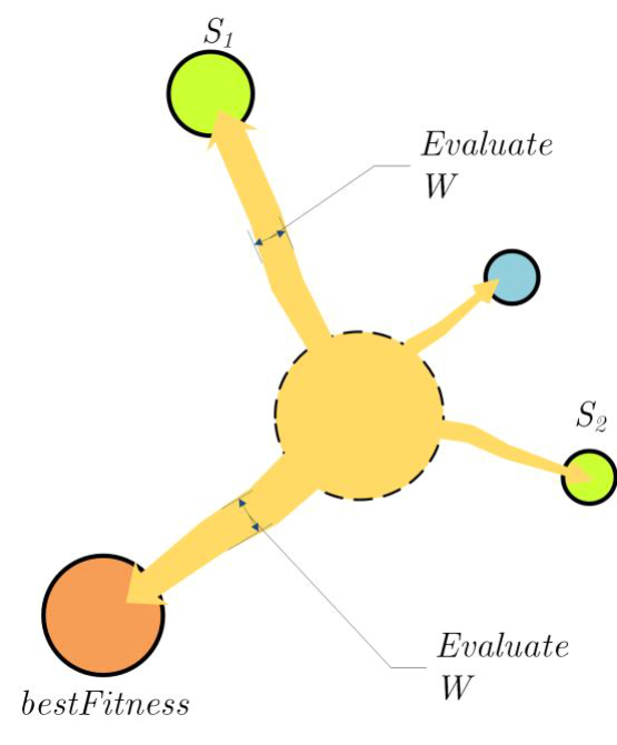
图 2.7.2-1 适应度评估(Assessment of fitness)(图片引子参考文献[1])
1)参数配置和模拟
SMA 算法实现迁移和更新于参考文献[2]和[3]的代码仓库②。为了解释算法的机制,将solutions(解)的维数定为易于观察的二维,表述为平面坐标系中的点。同时目标函数为简单的距离计算,代码如下:
  def objective_function(solution):
    food = np.array([50,50])
    result = np.linalg.norm(solution - food)

    return result
其中food = np.array([50,50])为搜寻的对象(食物),对应为点[50,50]。算法模拟提供了可调参数有迭代次数、最大问题或最小问题(试验问题为最小问题),及概率阈值p_t,和初始solutions(点)。输入多个点为起始条件的最小点数为5。执行Run(运行)完成计算,并将相关后续逐步解析所需的数据存入到本地磁盘空间,如图 2.7.2-2。
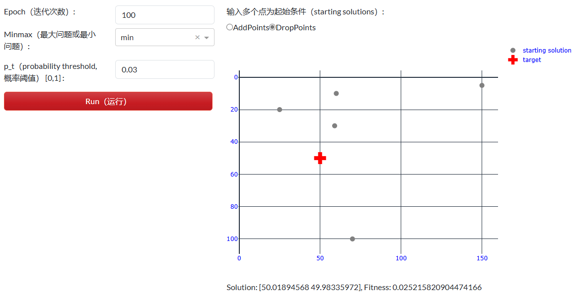
图 2.7.2-2 参数配置和模拟
图 2.7.2-2下方的Solution: [50.01894568 49.98335972], Fitness: 0.025215820904474166为执行Run(运行)后的结果,可以看到最优解为[50.018,49.983],基本同目标点[50,50],其适应度(Fitness)为 0.025,趋近于最小值0。
2)逐步解析
SMA 基本算法的伪代码如下:
Algorithm 1 Pseudo-code of SMA
Initialize the parameters popsize, Max_iteraition;
Initialize the positions of slime mould $X_i(i=1,2, \ldots, n)$;
While ( $t \leq$ Max_iteraition)
    Calculate the fitness of all slime mould;
    update bestFitness, $X_b$
    Calculate the $W$ by Eq. (2.5);
    For each search portion
        update $p, v b, v c$;
        update positions by Eq. (2.7);
    End For
    $t=t+1$;
End While
Return bestFitness, $X_b$;
试验中,参数popsize为starting solutions的维度(即种群的大小,多个解组成的集群称为种群population),为输入多个点的数量。Max_iteraition最大迭代次数可以根据全局最优曲线变化和fitness适应度结果来调整。
一个迭代周期中,
- 首先逐个计算每个点(agent)到目标点的距离(即由目标函数
objective_function()计算适应度); - 更新最佳适应度(bestFitness);
- 为每一个点(一个
solution解)的 x 和 y 值(solution解中的每个值,1维到多维的向量),计算权重(循环点计算)(公式2.5); - 更新参数 $p$, $\overrightarrow{v b}$ ,$\overrightarrow{v c}$(公式2.4,2.3);
- 由$p$为条件,以$\overrightarrow{v b} , \overrightarrow{v c}$为倍数,计算点更新的位置,即更新
solution(循环点更新)(公式2.1或2.7); - 开始下一个迭代。
实现 SMA 的原代码迁移于 Python 库mealpy③,具体位于bio_based->SMA.py④:
  #!/usr/bin/env python
# Created by "Thieu" at 20:22, 12/06/2020 ----------%
#       Email: nguyenthieu2102@gmail.com            %
#       Github: https://github.com/thieu1995        %
# --------------------------------------------------%

import numpy as np

import sys
import os

from ..optimizer import Optimizer


class DevSMA(Optimizer):
    """
    The developed version: Slime Mould Algorithm (SMA)

    Notes:
        + Selected 2 unique and random solution to create new solution (not to create variable)
        + Check bound and compare old position with new position to get the best one

    Hyper-parameters should fine-tune in approximate range to get faster convergence toward the global optimum:
        + p_t (float): (0, 1.0) -> better [0.01, 0.1], probability threshold (z in the paper)

    """

    def __init__(
        self,
        epoch: int = 10000,
        pop_size: int = 100,
        p_t: float = 0.03,
        **kwargs: object
    ) -> None:
        """
        Args:
            epoch (int): maximum number of iterations, default = 10000
            pop_size (int): number of population size, default = 100
            p_t (float): probability threshold (z in the paper), default = 0.03
        """
        super().__init__(**kwargs)
        self.epoch = self.validator.check_int("epoch", epoch, [1, 100000])
        self.pop_size = self.validator.check_int(
            "pop_size", pop_size, [5, 10000]
        )
        self.p_t = self.validator.check_float("p_t", p_t, (0, 1.0))
        self.set_parameters(["epoch", "pop_size", "p_t"])
        self.sort_flag = True

        if self.pickle_fn is None:
            self.pickle_fn = "processData/pData.pkl"

    def initialize_variables(self):
        self.weights = np.zeros((self.pop_size, self.problem.n_dims))

    def evolve(self, epoch):
        """
        The main operations (equations) of algorithm. Inherit from Optimizer class

        Args:
            epoch (int): The current iteration
        """
        self.processData_epoch = {}
        # plus eps to avoid denominator zero
        ss = (
            self.g_best.target.fitness
            - self.pop[-1].target.fitness
            + self.EPSILON
        )
        # calculate the fitness weight of each slime mold
        processData_epoch_weight = {
            "bF": self.g_best.target.fitness,
            "wF": self.pop[-1].target.fitness,
            "Si": [],
        }
        for idx in range(0, self.pop_size):
            # Eq.(2.5)
            if idx <= int(self.pop_size / 2):
                self.weights[idx] = 1 + self.generator.uniform(
                    0, 1, self.problem.n_dims
                ) * np.log10(
                    (self.g_best.target.fitness - self.pop[idx].target.fitness)
                    / ss
                    + 1
                )
            else:
                self.weights[idx] = 1 - self.generator.uniform(
                    0, 1, self.problem.n_dims
                ) * np.log10(
                    (self.g_best.target.fitness - self.pop[idx].target.fitness)
                    / ss
                    + 1
                )

            processData_epoch_weight["Si"].append(self.pop[idx].target.fitness)

        self.processData_epoch["weightEpoch"] = processData_epoch_weight

        a = np.arctanh(-(epoch / self.epoch) + 1)  # Eq.(2.4)
        b = 1 - epoch / self.epoch
        pop_new = []
        for idx in range(0, self.pop_size):
            # Update the Position of search agent
            if self.generator.uniform() < self.p_t:  # Eq.(2.7)
                pos_new = self.problem.generate_solution()
            else:
                p = np.tanh(
                    np.abs(
                        self.pop[idx].target.fitness
                        - self.g_best.target.fitness
                    )
                )  # Eq.(2.2)
                vb = self.generator.uniform(
                    -a, a, self.problem.n_dims
                )  # Eq.(2.3)
                vc = self.generator.uniform(-b, b, self.problem.n_dims)
                # two positions randomly selected from population, apply for the whole problem size instead of 1 variable
                id_a, id_b = self.generator.choice(
                    list(set(range(0, self.pop_size)) - {idx}), 2, replace=False
                )
                pos_1 = self.g_best.solution + vb * (
                    self.weights[idx] * self.pop[id_a].solution
                    - self.pop[id_b].solution
                )
                pos_2 = vc * self.pop[idx].solution
                condition = self.generator.random(self.problem.n_dims) < p
                pos_new = np.where(condition, pos_1, pos_2)
            # Check bound and re-calculate fitness after each individual move
            pos_new = self.correct_solution(pos_new)
            agent = self.generate_empty_agent(pos_new)
            pop_new.append(agent)
            if self.mode not in self.AVAILABLE_MODES:
                agent.target = self.get_target(pos_new)
                self.pop[idx] = self.get_better_agent(
                    agent, self.pop[idx], self.problem.minmax
                )
        if self.mode in self.AVAILABLE_MODES:
            pop_new = self.update_target_for_population(pop_new)
            self.pop = self.greedy_selection_population(
                self.pop, pop_new, self.problem.minmax
            )
观察每一个迭代由目标函数计算每个点适应度中最佳适应度的变化曲线(图 2.7.2-3)。并观察点的更新位置(图 2.7.2-4),即种群中每个agent更新后的solution解(试验中仅二维,根据分析问题可以为任意维度)。
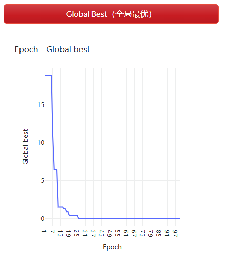
图 2.7.2-3 全局最优适应度
如果打开path on,可以观察每个点更新的路径。从更新路径中可以发现开始迭代时,更新点的跳动幅度较大,但是随着迭代的进行,幅度开始减小并趋向于目标点。这一变化与绘制曲线 a(arctanh),即值$\overrightarrow{v b}$ ,$\overrightarrow{v c}$的变化有关。
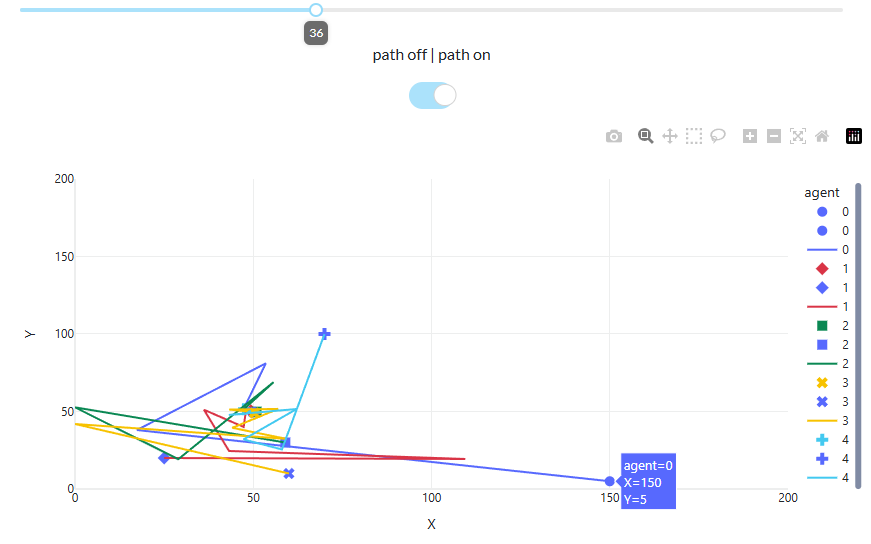
图 2.7.2-4 位置(solution)更新
以迭代epoch为一轴,对于每一个点 x 和 y 向的更新权重为另外两个轴的值(每个solution中各维度上的权重),观察每个点随迭代增加权重的变化,如图 2.7.2-5。
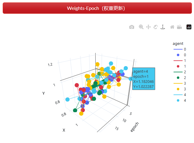
图 2.7.2-5 权重更新
每次迭代,根据各点的适应度,由解决的问题是最小还是最大问题排序种群中点的顺序。表 2.7.2-1中给出了各点(种群中的每个代理agent)适应度的排序。
表 2.7.2-1 最优排序索引
| agent_0 | agent_1 | agent_2 | agent_3 | agent_4 |
|---|---|---|---|---|
| 0 | 1 | 3 | 4 | 2 |
| 0 | 2 | 4 | 1 | 3 |
| 1 | 0 | 4 | 2 | 3 |
| 0 | 2 | 3 | 4 | 1 |
| 0 | 2 | 4 | 3 | 1 |
| 1 | 0 | 3 | 4 | 2 |
| 2 | 1 | 0 | 3 | 4 |
| 4 | 3 | 0 | 1 | 2 |
| 4 | 3 | 0 | 1 | 2 |
| 4 | 3 | 0 | 1 | 2 |
| 4 | 3 | 0 | 1 | 2 |
| 4 | 3 | 0 | 1 | 2 |
| 4 | 3 | 0 | 1 | 2 |
| 4 | 3 | 0 | 1 | 2 |
| 4 | 3 | 1 | 0 | 2 |
| 0 | 4 | 2 | 1 | 3 |
| 0 | 3 | 4 | 2 | 1 |
| 0 | 3 | 4 | 1 | 2 |
| 0 | 1 | 2 | 3 | 4 |
权重计算(公式 2.5),
$$ \begin{gathered} \overrightarrow{W(\text { SmellIndex }(i))}=\left\{\begin{array}{l} 1+r \cdot \log \left(\frac{b F-S(i)}{b F-w F}+1\right), \text { condition } \\ 1-r \cdot \log \left(\frac{b F-S(i)}{b F-w F}+1\right), \quad \text { others } \end{array}\right. \\ \text { SmellIndex }=\operatorname{sort}(S) \end{gathered} $$
权重公式中,$S(i)$为种群的一个解(solution);$bF$为当前迭代中最佳适应度;wF为当前迭代中最差适应度。$\frac{b F-S(i)}{b F-w F}$方法为 Min-Max scaling(最小-最大 标准化)方法,使解的值域缩放至[0,1]区间。log对数函数则将标准化后的值间的距离拉开(图 2.7.2-6),且趋向于最小值一端(左)的值间距离向最大值一端(右)开始拉大,即避免具有较好适应度的多个解的权重被拉开。其中condition的条件为,按适应度(fitness)排序种群后($sort(S)$),前后切分为两份,具有较好适应度部分的解权重值加1,否则用1去减,即具有较好适应度的解具有更高的权重值。
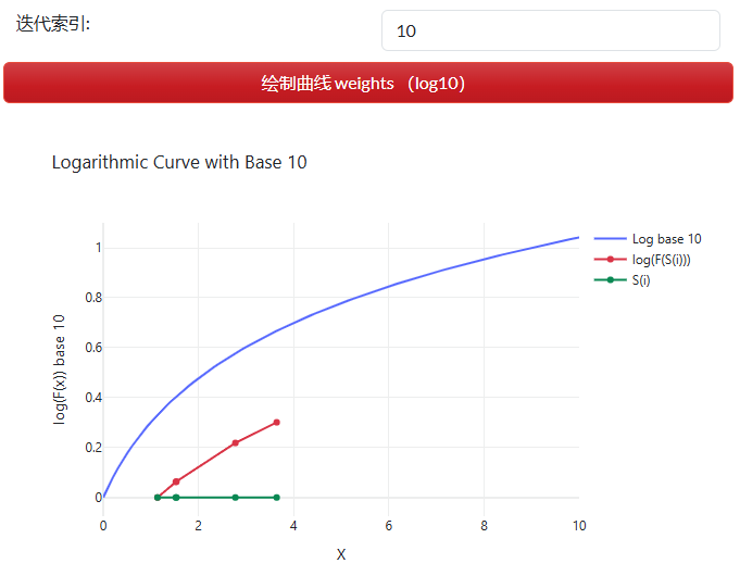
图 2.7.2-6 权重变化曲线
$p=\tanh |S(i)-D F|$ (公式 2.2)
式中,$S(i)$为一个解的适应度(目标函数返回值),$DF$为经过所有迭代后的最佳适应度(全局适应度)。$p$值表征了当前解到全局适应度的距离,用于公式 2.1 或 2.7 的条件。tanh函数将距离值缩放至[0,1]区间(如图 2.7.2-7),并拉开各个解之间的距离。当前解越接近于全局最优解,$p$值则越趋近于0,那么生成的随机数$r$,满足$r \geq p$的可能性越大,更多的是基于自身解的一个更新($\overrightarrow{v c} \cdot \overrightarrow{X(t)}$)。而当,当前解距离全局最优解较远,$p$值趋近于1,那么$r < p$的可能性很大,则更多的解更新使用公式$\overrightarrow{X_b(t)}+\overrightarrow{v b} \cdot\left(\vec{W} \cdot \overrightarrow{X_A(t)}-\overrightarrow{X_B(t)}\right)$, 是放弃当前解,而基于当前迭代最优解来更新。
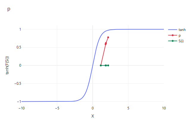
图 2.7.2-7 绘制曲线$p$
$a=\operatorname{arctanh}\left(-\left(\frac{t}{\max _{-} t}\right)+1\right)$ (公式 2.4)
$\overrightarrow{v b}=[-a, a]$ (公式 2.3)
$b=1-\left(\frac{t}{\max _{-} t}\right)$
$\overrightarrow{v c}=[-b, b]$
每次迭代时,当前解更新的步幅究竟为多大,对应变量$\overrightarrow{v c}$和$\overrightarrow{v b}$,其与迭代次数相关,如绘制曲线a (arctanh)(图 2.7.2-8),当迭代次数增加,变化步幅则逐步减少。$b$为一条斜线,值域[0,1];而$a$在开始迭代时具有较大的值,即$\overrightarrow{v b}$的区间较大,那么更新的步幅会出现较大的可能性,该种情况主要针对开始迭代期间,当前解不理想的情况。
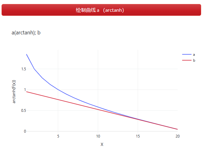
图 2.7.2-8 绘制曲线$a, b$
  Latex bak
$$
\overrightarrow{X(t+1)}=\left\{\begin{array}{c}
\overrightarrow{X_b(t)}+\overrightarrow{v b} \cdot\left(\vec{W} \cdot \overrightarrow{X_A(t)}-\overrightarrow{X_B(t)}\right), r<p \\
\overrightarrow{v c} \cdot \overrightarrow{X(t)}, r \geq p
\end{array}\right.
$$
$$ \overrightarrow{X(t+1)} = \begin{cases} \overrightarrow{X_b(t)} + \overrightarrow{v b} \cdot \left( \vec{W} \cdot \overrightarrow{X_A(t)} - \overrightarrow{X_B(t)} \right), & r < p \ \overrightarrow{v c} \cdot \overrightarrow{X(t)}, & r \geq p \end{cases} (公式 2.1) $$
  Latex bak
$$
\overrightarrow{X^*}=\left\{\begin{array}{l}
\text { rand } \cdot(U B-L B)+L B, \text { rand }<z \\
\overrightarrow{X_b(t)}+\overrightarrow{v b} \cdot\left(W \cdot \overrightarrow{X_A(t)}-\overrightarrow{X_B(t)}\right), r<p \\
\overrightarrow{v c} \cdot \overrightarrow{X(t)}, r \geq p
\end{array}\right.
$$
$$ \overrightarrow{X^*} = \begin{cases} \text{rand} \cdot (UB - LB) + LB, & \text{rand} < z \ \overrightarrow{X_b(t)} + \overrightarrow{v b} \cdot \left( W \cdot \overrightarrow{X_A(t)} - \overrightarrow{X_B(t)} \right), & r < p \ \overrightarrow{v c} \cdot \overrightarrow{X(t)}, & r \geq p \end{cases} (公式 2.7) $$
由条件$p$,选择更新的方式,当前解趋向于全局最优解时,更多依据自身解更新;否则,更多依据当前最优解,和从种群中随机选择的两个解之间的距离进行更新(包含权重的影响)。
$\overrightarrow{v c}$是[0,1]区间的一个随机数,且随着迭代次数的增加,区间$[-a,a]$的宽度逐步缩小。
Daisy——算法交互图解代码托管于 GitHub,地址为 daisy⑤。
2.7.2.2 建立 SMA 组件
因为 Python script 可以安装 Python 库,因此可以直接迁移实现元启发式算法(meta-heuristic algorithms)的库。前文Daisy 算法交互图解①即迁移了mealpy③库,因为需要修改部分参数,实现源码中未提供的功能,因此未直接调用该库,而是选择性的迁移代码,融合到daisy⑤下。将 SMA 等元启发式算法写成 GH 组件,采取了类似的方式。首先,将 mealpy 库选择性的迁移到moths⑥库下,能够实现 mealpy 库中 SMA 等算法的计算。在 Rhino Python 环境下(PowerShell中)通过pip install moths安装(详细解释见 2.1 部分PyPI 包)。然后,在 GH 的 Python script 编辑器中调入该库的方法,方便建立 SMA 组件,而不用从零开始开发,结果图 2.7.2-9。

图 2.7.2-9 SMA 组件集
Moths 中集成的 SMA 是纯粹的 Python 代码,不能直接与 RH 或者 GH 中的(几何)元素交互。为了实现与 GH 输入输出端衔接并可以控制部分参数,定义了3-HeuristicOptimizer优化器组件,主体代码迁移于源代码中的optimizer.py模块,在其track_optimize_step()方法中添加了print(f">>>Problem:...)语句,当输入端Verbose参数为True时,输出该信息,用于解算相关信息查看。可以看到类Optimizer所用到的依赖库部分直接从moths库中调用,而不是将其全部迁移到 GH 环境下。输出端的变量即为类Optimizer,作为其它算法类的父类,这里是SMA类。
3-HeuristicOptimizer (Python Script 组件)
  import numpy as np
from typing import List, Union, Tuple, Dict
from moths.heuristic_algorithms.utils.agent import Agent
from moths.heuristic_algorithms.utils.problem import Problem
from math import gamma
from moths.heuristic_algorithms.utils.history import History
from moths.heuristic_algorithms.utils.target import Target
from moths.heuristic_algorithms.utils.termination import Termination
from moths.heuristic_algorithms.utils.logger import Logger
from moths.heuristic_algorithms.utils.validator import Validator
import concurrent.futures as parallel
from functools import partial
import os
import time

ghenv.Component.Name = '3-HeuristicOptimizer'
ghenv.Component.NickName = '3-HeuristicOptimizer'
ghenv.Component.Description = '元启发式算法优化器'
ghenv.Component.Message = '0.0.1'
ghenv.Component.Category = 'Moths'
ghenv.Component.SubCategory = 'Algorithm N Design'
ghenv.Component.PanelSection = 3

class Optimizer:
    """
    The base class of all algorithms. All methods in this class will be inherited

    Notes
    ~~~~~
    + The function solve() is the most important method, trained the model
    + The parallel (multithreading or multiprocessing) is used in method: generate_population(), update_target_for_population()
    + The general format of:
        + population = [agent_1, agent_2, ..., agent_N]
        + agent = [solution, target]
        + target = [fitness value, objective_list]
        + objective_list = [obj_1, obj_2, ..., obj_M]
    """

    EPSILON = 10E-10
    SUPPORTED_MODES = ["process", "thread", "swarm", "single"]
    AVAILABLE_MODES = ["process", "thread", "swarm"]
    PARALLEL_MODES = ["process", "thread"]
    SUPPORTED_ARRAYS = [list, tuple, np.ndarray]

    def __init__(self, **kwargs):

    def __set_keyword_arguments(self, kwargs):

    def set_parameters(self, parameters: Union[List, Tuple, Dict]) -> None:

	def get_parameters(self) -> Dict:

    def get_attributes(self) -> Dict:

    def get_name(self) -> str:

    def __str__(self):

    def initialize_variables(self):

    def before_initialization(self, starting_solutions: Union[List, Tuple, np.ndarray] = None) -> None:

    def initialization(self) -> None:

    def after_initialization(self) -> None:

    def before_main_loop(self):

    def evolve(self, epoch: int) -> None:

    def check_problem(self, problem, seed) -> None:

    def check_mode_and_workers(self, mode, n_workers):

    def check_termination(self, mode="start", termination=None, epoch=None):

    def solve(self, problem: Union[Dict, Problem] = None, mode: str = 'single', n_workers: int = None,
              termination: Union[Dict, Termination] = None, starting_solutions: Union[List, np.ndarray, Tuple] = None,
              seed: int = None) -> Agent:
        """
        Args:
            problem: an instance of Problem class or a dictionary
            mode: Parallel: 'process', 'thread'; Sequential: 'swarm', 'single'.

                * 'process': The parallel mode with multiple cores run the tasks
                * 'thread': The parallel mode with multiple threads run the tasks
                * 'swarm': The sequential mode that no effect on updating phase of other agents
                * 'single': The sequential mode that effect on updating phase of other agents, this is default mode

            n_workers: The number of workers (cores or threads) to do the tasks (effect only on parallel mode)
            termination: The termination dictionary or an instance of Termination class
            starting_solutions: List or 2D matrix (numpy array) of starting positions with length equal pop_size parameter
            seed: seed for random number generation needed to be *explicitly* set to int value

        Returns:
            g_best: g_best, the best found agent, that hold the best solution and the best target. Access by: .g_best.solution, .g_best.target
        """
        self.check_problem(problem, seed)
        self.check_mode_and_workers(mode, n_workers)
        self.check_termination("start", termination, None)
        self.initialize_variables()

        self.before_initialization(starting_solutions)
        self.initialization()
        self.after_initialization()

        self.before_main_loop()
        for epoch in range(1, self.epoch + 1):
            # print(f"Epoch:{epoch}")
            time_epoch = time.perf_counter()

            # Evolve method will be called in child class
            self.evolve(epoch)

            # Update global best solution, the population is sorted or not depended on algorithm's strategy
            pop_temp, self.g_best = self.update_global_best_agent(self.pop)
            if self.sort_flag: self.pop = pop_temp

            time_epoch = time.perf_counter() - time_epoch
            self.track_optimize_step(self.pop, epoch, time_epoch)
            if self.check_termination("end", None, epoch):
                break

        self.track_optimize_process()
        return self.g_best

    def track_optimize_step(self, pop: List[Agent] = None, epoch: int = None, runtime: float = None) -> None:
        """
        Save some historical data and print out the detailed information of training process in each epoch

        Args:
            pop: the current population
            epoch: current iteration
            runtime: the runtime for current iteration
        """
        # Save history data
        if self.problem.save_population:
            self.history.list_population.append(Optimizer.duplicate_pop(pop))
        self.history.list_epoch_time.append(runtime)
        self.history.list_global_best_fit.append(self.history.list_global_best[-1].target.fitness)
        self.history.list_current_best_fit.append(self.history.list_current_best[-1].target.fitness)
        # Save the exploration and exploitation data for later usage
        pos_matrix = np.array([agent.solution for agent in pop])
        div = np.mean(np.abs(np.median(pos_matrix, axis=0) - pos_matrix), axis=0)
        self.history.list_diversity.append(np.mean(div, axis=0))
        # Print epoch
        self.logger.info(f">>>Problem: {self.problem.name}, Epoch: {epoch}, Current best: {self.history.list_current_best[-1].target.fitness}, "
                         f"Global best: {self.history.list_global_best[-1].target.fitness}, Runtime: {runtime:.5f} seconds")
        if Verbose:
            print(f">>>Problem: {self.problem.name}, Epoch: {epoch}, Current best: {self.history.list_current_best[-1].target.fitness}, "
                            f"Global best: {self.history.list_global_best[-1].target.fitness}, Runtime: {runtime:.5f} seconds")

    def track_optimize_process(self) -> None:

    def generate_empty_agent(self, solution: np.ndarray = None) -> Agent:

    def generate_agent(self, solution: np.ndarray = None) -> Agent:

    def generate_population(self, pop_size: int = None) -> List[Agent]:

    def amend_solution(self, solution: np.ndarray) -> np.ndarray:

    def correct_solution(self, solution: np.ndarray) -> np.ndarray:

    def update_target_for_population(self, pop: List[Agent] = None) -> List[Agent]:

    def get_target(self, solution: np.ndarray, counted: bool = True) -> Target:

    @staticmethod
    def compare_target(target_x: Target, target_y: Target, minmax: str = "min") -> bool:

    @staticmethod
    def compare_fitness(fitness_x: Union[float, int], fitness_y: Union[float, int], minmax: str = "min") -> bool:

    @staticmethod
    def duplicate_pop(pop: List[Agent]) -> List[Agent]:

    @staticmethod
    def get_sorted_population(pop: List[Agent], minmax: str = "min", return_index: bool = False) -> List[Agent]:

    @staticmethod
    def get_best_agent(pop: List[Agent], minmax: str = "min") -> Agent:

    @staticmethod
    def get_index_best(pop: List[Agent], minmax: str = "min") -> int:

    @staticmethod
    def get_worst_agent(pop: List[Agent], minmax: str = "min") -> Agent:

    @staticmethod
    def get_special_agents(pop: List[Agent] = None, n_best: int = 3, n_worst: int = 3,

    @staticmethod
    def get_special_fitness(pop: List[Agent] = None, minmax: str = "min") -> Tuple[Union[float, np.ndarray], float, float]:

    @staticmethod
    def get_better_agent(agent_x: Agent, agent_y: Agent, minmax: str = "min", reverse: bool = False) -> Agent:

    @staticmethod
    def greedy_selection_population(pop_old: List[Agent] = None, pop_new: List[Agent] = None, minmax: str = "min") -> List[Agent]:

    @staticmethod
    def get_sorted_and_trimmed_population(pop: List[Agent] = None, pop_size: int = None, minmax: str = "min") -> List[Agent]:

	def get_index_roulette_wheel_selection(self, list_fitness: np.array):

    def get_index_kway_tournament_selection(self, pop: List = None, k_way: float = 0.2, output: int = 2, reverse: bool = False) -> List:

    def get_levy_flight_step(self, beta: float = 1.0, multiplier: float = 0.001,

    def generate_opposition_solution(self, agent: Agent = None, g_best: Agent = None) -> np.ndarray:

    def generate_group_population(self, pop: List[Agent], n_groups: int, m_agents: int) -> List:

    def crossover_arithmetic(self, dad_pos=None, mom_pos=None):

    def improved_ms(self, pop=None, g_best=None):  ## m: mutation, s: search

if __name__=="__main__":
    Optimizer = Optimizer
SMA 是算法核心,定义组件3-SMA的核心代码迁移于源代码SMA.py模块,其类DevSMA(Optimizer)的父类为Optimizer(以输入端参数的方式调入)。并将类初始化条件epoch、pop_size、p_t和starting_solutions引出为组件的输入端参数。输出参数为类DevSMA初始化参数的实例化对象。
3-SMA (Python Script 组件)
  import numpy as np

ghenv.Component.Name = "3-SMA"
ghenv.Component.NickName = "3-SMA"
ghenv.Component.Description = "SMA——黏菌算法"
ghenv.Component.Message = "0.0.1"
ghenv.Component.Category = "Moths"
ghenv.Component.SubCategory = "Algorithm N Design"
ghenv.Component.PanelSection = 3


class DevSMA(Optimizer):

    def __init__(
        self,
        epoch: int = 10000,
        pop_size: int = 100,
        p_t: float = 0.03,
        **kwargs: object
    ) -> None:

    def initialize_variables(self):

    def evolve(self, epoch):

if __name__ == "__main__":
    if Epoch and Pop_size:
        if Starting_solutions is not None:
            starting_solutions = [[pt[0], pt[1]] for pt in Starting_solutions]

            SMA = DevSMA(
                epoch=Epoch,
                pop_size=len(Starting_solutions),
                p_t=P_t,
                starting_solutions=starting_solutions,
            )
        else:
            SMA = DevSMA(epoch=Epoch, pop_size=Pop_size, p_t=P_t)
通过优化器和实现 SMA 算法的类完成初始条件配置后,根据所要解决的问题配置problem_dict参数,包括解(solution)的边界条件bounds,求解方向minmax和目标函数obj_func,定义组件3-SMAMetaHeuristicSolving实现。但在组件定义时,将目标函数作为输入端参数传入,以方便灵活定义目标函数。
3-SMAMetaHeuristicSolving (Python Script 组件)
  """
    配置 HeuristicOptimizer(优化器)和 SMA 后,指定解的区间(LB 和 UB)及解的方向(MinMax),最大值还是最小值,给定目标函数求解
    Inputs:
        SMA: Item Access; No Type Hint
            SMA 类的实例化对象
        LB: List Access; float
            解的最小值列表,对应维度
        UB: List Access; float
            解的最大值列表,对应维度
        MinMax: Item Access; str
            求解方向,min 或 max
        ObjectionveFunction: Item Access; No Type Hint
            目标函数
        Run: Item Access; bool
            是否运行求解
    Output:
        Verbose: Item; str
            打印输出的字符串。结算信息
        Solution: List; float
            最优解
        Fitness: Item; flaot
            适应度

"""

from moths.heuristic_algorithms.utils.space import FloatVar

ghenv.Component.Name = "3-SMAMetaHeuristicSolving"
ghenv.Component.NickName = "3-SMAMetaHeuristicSolving"
ghenv.Component.Description = "SMA——元启发式算法解算"
ghenv.Component.Message = "0.0.1"
ghenv.Component.Category = "Moths"
ghenv.Component.SubCategory = "Algorithm N Design"
ghenv.Component.PanelSection = 3


if __name__ == "__main__":
    if hasattr(SMA, "starting_solutions"):
        dimension = 2
    elif Dimension:
        dimension = Dimension
    else:
        dimension = 1

    if ObjectionveFunction:
        problem_dict = {
            "bounds": FloatVar(
                lb=LB * dimension, ub=UB * dimension, name="delta"
            ),
            "minmax": MinMax,
            "obj_func": ObjectionveFunction,
        }

        if Run:
            g_best = SMA.solve(problem_dict)

            Solution = list(SMA.g_best.solution)
            Fitness = SMA.g_best.target.fitness
目标函数是要根据所要解决的问题来定义。如图 2.7.2-10 为给定一个曲线,在曲线上指定区间内选择4个点,这4个点围合的面积趋近于指定的值,求解这4个点对应曲线的参数值。这个问题是典型的最小值问题,可以用 SMA 求解。根据问题定义目标函数objective_function(),并作为输出端参数值,定义组件3-ObjFunc-FindPolygon实现。
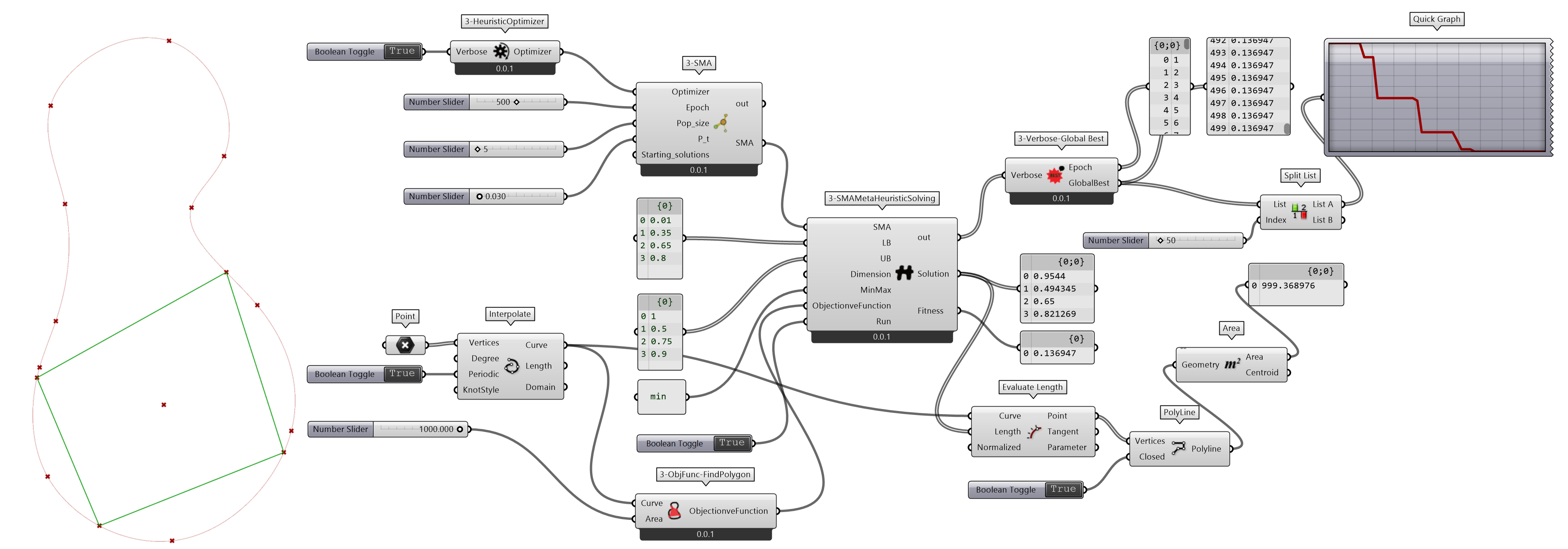
图 2.7.2-10 用 SMA 求解点围合的面积趋向于指定值
3-ObjFunc-FindPolygon (Python Script 组件)
  """
    在曲线上寻找4个点,使得围合的面积趋向于指定的目标面积
    Inputs:
        Curve: Item Access; Curve
            输入的曲线
        Area: Item Access; float
            趋向于的目标面积
    Output:
        ObjectionveFunction: Function
            目标函数

"""

import numpy as np
import rhinoscriptsyntax as rs
import Rhino.Geometry as rg

ghenv.Component.Name = "3-ObjFunc-FindPolygon"
ghenv.Component.NickName = "3-ObjFunc-FindPolygon"
ghenv.Component.Description = (
    "在曲线上寻找4个点,使得围合的面积趋向于指定的目标面积"
)
ghenv.Component.Message = "0.0.1"
ghenv.Component.Category = "Moths"
ghenv.Component.SubCategory = "Algorithm N Design"
ghenv.Component.PanelSection = 3


def objective_function(solution):
    curveLength = rs.CurveLength(Curve)
    pts = [rs.EvaluateCurve(Curve, param * curveLength) for param in solution]
    polyline = rs.AddPolyline(pts + [pts[0]])
    polylineArea = rs.Area(polyline)

    return abs(Area - polylineArea)


if __name__ == "__main__":
    ObjectionveFunction = objective_function
为了观察全局最优解适应度值的变化,定义组件3-Verbose-Global Best提取解算过程中输出的信息迭代次数Epoch和全局最优解适应度值GlobalBest,而后用组件Quick Graph查看值变化曲线。
3-Verbose-Global Best (Python Script 组件)
  """
    从打印输出的字符串中提取信息,查看全局最优解
    Inputs:
        Verbose: Item Access; str
            打印输出的字符串
    Output:
        Epoch: List; int
            迭代次数
        GlobalBest: List; float
            全局最优解
"""

import re

ghenv.Component.Name = "3-Verbose-Global Best"
ghenv.Component.NickName = "3-Verbose-Global Best"
ghenv.Component.Description = "查看全局最优解"
ghenv.Component.Message = "0.0.1"
ghenv.Component.Category = "Moths"
ghenv.Component.SubCategory = "Algorithm N Design"
ghenv.Component.PanelSection = 3

if Verbose:
    match = re.search(r">>>(.*)", Verbose)
    parsed_entries = []
    if match:
        key_value_str = match.group(1).strip()
        pairs = [kv.strip() for kv in key_value_str.split(",")]
        key_value_dict = {
            k.strip(): v.strip() for k, v in (kv.split(":") for kv in pairs)
        }
        parsed_entries.append(key_value_dict)

        Epoch = int(key_value_dict["Epoch"])
        GlobalBest = float(key_value_dict["Global best"])
注释(Notes):
① Daisy 算法交互图解,(https://daisy-codingx.pythonanywhere.com/meta_heuristic/SMA)。
② 参考文献[2]和[3]的代码仓库,元启发式算法(https://github.com/thieu1995/metaheuristics)。
③ mealpy,是世界上最大面向大多数前沿元启发式算法(meta-heuristic algorithms)(自然启发算法(nature-inspired algorithms)、黑盒优化(black-box optimization)、全局搜索优化器(global search optimizers)、迭代学习算法( iterative learning algorithms)、连续优化(continuous optimization)、导数自由优化(derivative free optimization)、梯度自由优化(gradient free optimization)、零阶优化(zeroth order optimization)、随机搜索优化(stochastic search optimization)、随机搜索优化(random search optimization))的 Python 库。这些算法属于基于种群的算法(population-based algorithms,PMA),为近似优化(approximate optimization)领域中最流行的算法。(https://pypi.org/project/mealpy/)。
④ bio_based->SMA.py,黏菌算法代码模块(https://github.com/thieu1995/mealpy/blob/master/mealpy/bio_based/SMA.py)。
⑤ daisy,Daisy 算法交互图解代码仓库(https://github.com/richieBao/daisy)。
⑥ moths,为 Grasshopper 参数化设计模组 moths 的支持工具。本书开发的 Python 库工具(https://github.com/richieBao/moths_PyPI)。
参考文献:
[1] Li, S., Chen, H., Wang, M., Heidari, A. A., & Mirjalili, S. (2020). Slime mould algorithm: A new method for stochastic optimization. Future Generation Computer Systems, 111, 300–323. doi:10.1016/j.future.2020.03.055.
[2] Nguyen, T., Tran, N., Nguyen, B. M., & Nguyen, G. (2018, November). A Resource Usage Prediction System Using Functional-Link and Genetic Algorithm Neural Network for Multivariate Cloud Metrics. In 2018 IEEE 11th Conference on Service-Oriented Computing and Applications (SOCA) (pp. 49-56). IEEE.
[3] Nguyen, T., Nguyen, B. M., & Nguyen, G. (2019, April). Building Resource Auto-scaler with Functional-Link Neural Network and Adaptive Bacterial Foraging Optimization. In International Conference on Theory and Applications of Models of Computation (pp. 501-517). Springer, Cham.